I first learned about this paper when Google Brain released the Tensorflow Recommenders library last month. I focused on it because Google, which operates a massive recommendation system like YouTube, was releasing recommendation system-related code. The overall content is more detailed in the Tensorflow Blog, so please read it.
The goals of TFRS (TensorFlow Recommenders) are as follows:
- Build recommendation candidates quickly and flexibly
- Structure that freely uses Item, User, Context information
- Multi-task structure that learns various objectives simultaneously
- Learned models are efficiently served through TF Serving
Actually, the code itself doesn’t have much diverse content, but what was most impressive was the Two Tower Model introduced as the basic model in the code. It’s about training User and Item completely independently and only predicting click/unclick with dot product at the final stage. The more I think about it, the better the structure seems. Although it’s unknown whether it will show tremendous performance since user tower and item tower can’t interact during training, the structure itself has no constraints on input features, so you can freely add possible features, and during inference, you can serve efficiently by having user embeddings and item embeddings and calculating similarity only with dot product, so compatibility with ANN (Approximate Nearest Neighbors) libraries also looks good.

Source: https://blog.tensorflow.org/2020/09/introducing-tensorflow-recommenders.html
Another advantage is that you can put meta information. A common problem in recommendation systems is the cold start problem. Whether it’s an Item or User, when there’s no usage history initially, you have to rely on meta information, and it’s difficult to model this universally well. However, the above two tower model can immediately start modeling by putting User or Item meta information and putting average values for the rest, even without usage history, so it seems like the cold start problem can be solved naturally. This also means it can be used well in structures where the item pool changes dynamically.
Thinking this far, I read and summarized the Two Tower Model related paper in more detail. The original paper title is “Sampling-Bias-Corrected Neural Modeling for Large Corpus Item Recommendations”, published by Google Brain in YouTube, and it’s the model currently used in candidate generation in the YouTube recommendation system.
1. Concept
YouTube recommendations are largely divided into 2 stages. These are candidate generation and ranking model. When recommending which video to which user, 1) candidate generation filters out a few hundred items worth recommending from all items, and 2) ranking model decides which few will go to the final recommendation. Here, candidate generation is important for recall@k since the actual desired item must be in the recommendation candidate pool, and ranking model is important for nDCG@k, HR@k since the actual desired item must be ranked at the top.
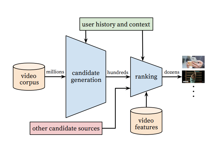
Also, thinking from the perspective of actually building a recommendation system, candidate generation model needs to filter a few hundred from all items, so moderate performance and fast inference speed are more important than the best performance. The method to make inference fast and filter a few hundred from hundreds~tens of millions of items is to extract good embedding vectors of items and find items similar to items recently consumed by the user as candidates.
The way to extract some item’s embedding can be as simple as combining word2vec and bag of words to extract text embedding of the item, or for videos or images, you can extract low-dimensional features using pretrained image models. The two tower model proposed in this paper is used by putting meta information and various features to create good user/item embeddings and then finding nearest neighbors based on dot distance.
2. Modeling Overview
Then let’s look at the two tower structure that’s central to this paper, and how this paper only had positive pairs at the data level and drew negative samples within batches.
Two-tower Model
Actually, two tower model first became popular as dual encoder in the natural language processing field. In tasks where you want to predict the relationship between two sentences, you put each sentence through an encoder and classify the relationship of sentences using the sentence representation that comes out. Here, encoders used range from RNN, Transformer to recently pretrained BERT structures. The key point of this structure is that when there are infinitely many labels to classify, instead of approaching it as multi-label classification, you approach it as binary classification by inputting query and label to judge whether it’s suitable or not.
Batch Negative Sampling
When learning a Two-tower model, the data needed is data that some user clicked an item and data that some user saw but didn’t click an item. However, there are several difficulties that can arise when collecting this “didn’t click” data, as follows:
- You might not be able to get data that says “was exposed” depending on the service environment.
- Data size: Usually, the number of impressions (exposures) is overwhelmingly more than clicks. If you start storing this, the data size becomes excessively large.
- Serving bias: unclick is entirely determined by what the recommendation logic was at the time. Therefore, the data distribution of negatives varies greatly according to the recommendation logic.
- Hard negative: Exposure is also ultimately the result of failures among the topk recommendations from existing logic, and the fact that it was exposed as topk from existing logic itself is already a difficult negative.
To solve this, batch negative sampling is randomly drawing negatives within batches when learning with only click data. When positive pairs come in batch units, you map different items to the user by changing the order, and think of this as negative. In Two Tower models, you can proceed with batch negative sampling right before the final dot product to avoid duplicate calculations.
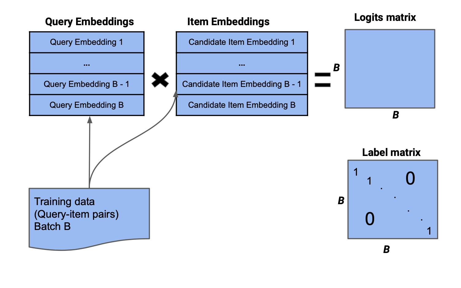
In the above figure, when you do matmul calculation with query embedding and item embedding, you get a label matrix, and only the $(i,i)$ column is positive and the rest are all negative. You don’t use everything as negative, and there are several basic methods for negative sampling. Representative ones are as follows:
- random negative: randomly sample k out of $B$-1.
- hard negative: only sample the pairs that the model found most difficult (those with the highest dot product values) out of $B$-1.
- semi-hard negative: sample k out of pairs that the model found somewhat difficult (those with dot product values in a specific range) out of $B$-1.
If you proceed with such negative sampling in the final stage of the two-tower model, there’s no guarantee that performance will definitely be good, but at least the data size decreases to a few tenths, and since the calculation isn’t much different from before, learning speed increases by several tens of times.
However, there aren’t only good points. As mentioned earlier, batch negative sampling is used in many fields besides recommendation, but there’s a problem that occurs when doing batch negative sampling in recommendation. It’s popular items. In recommendation, the probability of items appearing is very skewed toward certain popular ones. Since that means many clicks occur, it doesn’t matter when looking at positive samples, but the problem is that there are too many popular items in negative candidate groups when doing negative sampling. This is called item frequency bias. This paper solves this by estimating the sampling probability for each item and subtracting it from the matmul logit. This way, loss for popular items automatically decreases.
3. Stream Frequency Estimation
Then how can we calculate the probability that each item will be sampled in batches? It’s about quickly estimating the popularity of the item over time, but this is more difficult than expected. Even for the same item, popularity can surge over time, or conversely, it can suddenly disappear. The paper calculated this with a simple algorithm.
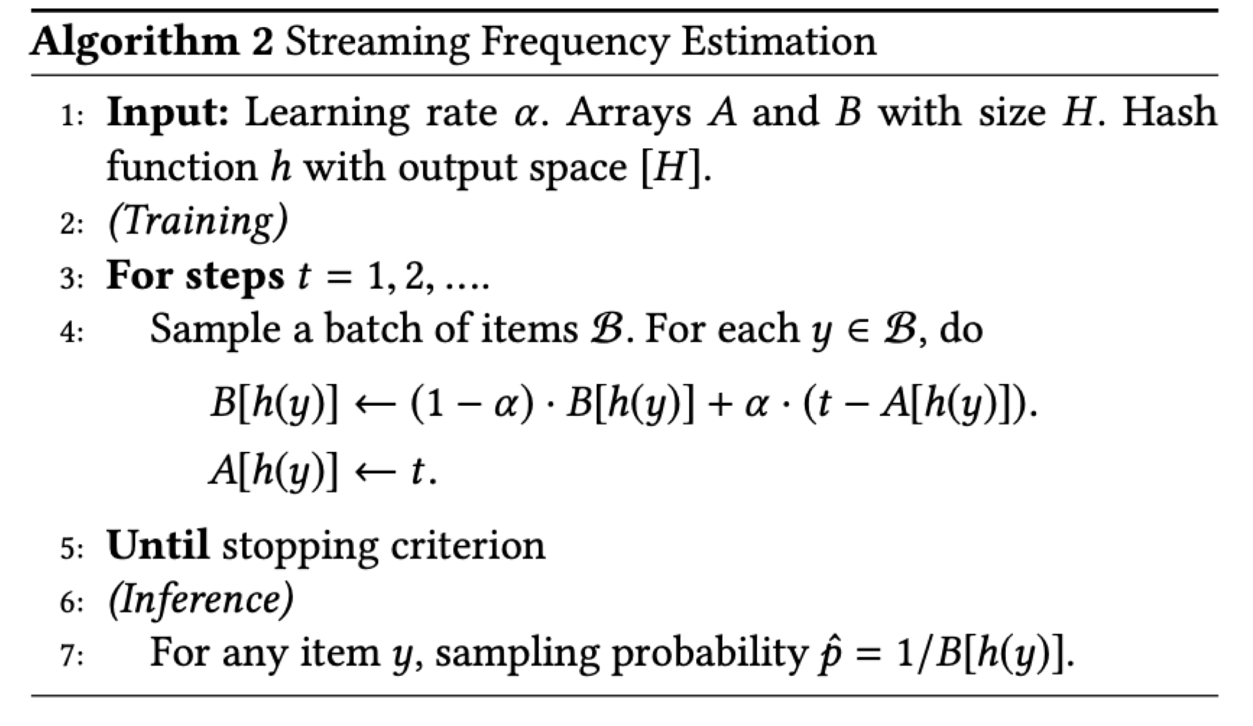
In the above equation, $h(y)$ is a function that hashes $y$ item id since it can increase infinitely, and $A[h(y)]$ is information about how many batches ago $y$ appeared. If it appeared in the immediately previous batch, it’s 1, and if it never appeared, it becomes $t$. That is, it’s information indicating how recently it was sampled.
For items that appear in each batch, you calculate the current sampling probability using information about how recently it was sampled and the previously stored sampling probability. The previously calculated sampling probability is time decayed by $(1-\alpha)$ and updated reflecting recency. Based on this, you calculate the sampling probability of a specific item in situations where the item appearance probability changes dynamically.
This is the main theoretical content of the paper, and from now on, let’s look at what features were used together and how it was used in actual YouTube recommendations.
4. Youtube Neural Retrieval Models
Features
As mentioned in 1. Concept, two-tower model is used in candidate generation in YouTube. Each feature is as follows:
- training label: Only use positive, but learn with 0 for clicks with little viewing and 1 for clicks with much viewing.
- Item features: Use video_id, channel_id, etc., and each is converted to trainable dense features through embedding lookup.
- User features: Take embeddings of several recently viewed video ids and average them.
The common point here is that video_ids are converted to trainable dense vectors similar to word embeddings.
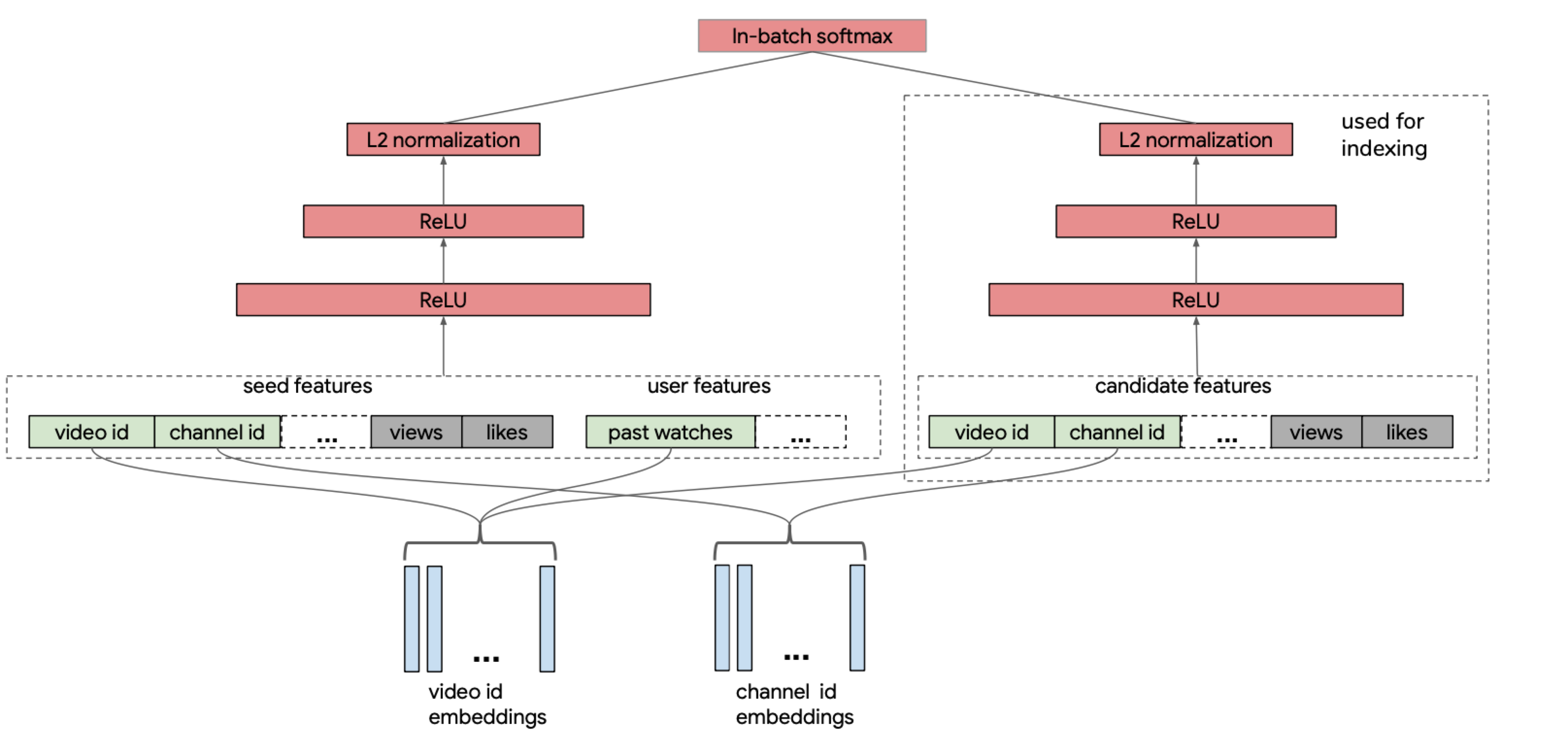
Besides this, information like view, like of the item also goes in, but it’s not revealed exactly how it was scaled, but you can guess it was scaled to 0~1 by referring to the 16-year YouTube recommendation paper.
Sequential Training
Then what size data was learned and at what cycle? YouTube says they receive one day’s data and learn once a day. The peculiar point is that unlike general deep learning training, they only do 1 epoch and don’t shuffle. The reason for not shuffling is to catch data distribution shift since the data distribution changes so much over time.