Recently, while studying Recommender Systems, I thought I needed to study the field of Multi-armed bandit. I’ve summarized it based on A Survey of Online Experiment Design with the Stochastic Multi-Armed Bandit.
Table of Contents
1. Concept
The background of the term Multi-armed Bandit (hereinafter MAB) is gambling. What is the method for someone to obtain maximum profit through N slot machines with different profit distributions within a given time? If given the opportunity to pull N slot machines within limited time to obtain profit, there should first be a process of exploring which slot machine can earn more money for some time (this is called Exploration), and then there is a process of maximizing profit by pulling slot machines that one judges to be good (this is called Exploitation).
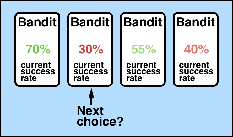
If you do a lot of exploration, you can better understand which slot machine has a higher success probability, but there’s a disadvantage that you only search for it and don’t actually earn much profit. If you do a lot of exploitation, you can get decent profit among known distributions, but you’ll regret not trying to find a better slot machine. This is called the exploration-exploitation tradeoff.
MAB makes decisions for fast judgment and good results while properly controlling this exploration-exploitation tradeoff. From the perspective that it learns while interacting with the environment and makes decisions, it can be considered a type of reinforcement learning. It is used in recommendation systems, stock investment, medical experiments, etc.
The biggest difference from existing Supervised Learning is that we put resources (time, number of attempts, etc.) as variables in real-time exploration & exploitation. Existing Supervised learning has a fixed problem, collects data corresponding to that problem, and then finds a decision boundary to predict the value to be predicted. However, in stock investment or recommendation systems, the value to be predicted often changes, so the process of collecting data, learning, and predicting through it often takes too long. Therefore, one of the methodologies to obtain the best profit within limited resources is Multi Armed Bandit.
2. Differences between MAB and Existing Statistical Models
MAB experimental environments are mostly cases where you can receive results immediately from some attempt. Therefore, before learning about MAB algorithms, the first thing to think about is how to evaluate algorithms in MAB experimental environments. Existing supervised learning or unsupervised learning has a clear loss function and the goal is to minimize it. However, in MAB experimental environments, unless you evaluate directly in the actual online environment (in fact, this isn’t complete either), it’s difficult to evaluate what performance the MAB algorithm has. This is measured through regret, variance and bounds of regret, stationary, feedback delay.
1) Regret
Regret is easier to understand in its dictionary meaning. It’s how much I’ll regret when I check the results later after making a choice.
“The remorse(losses) felt after the fact as a result of dissatisfaction with the agent’s (prior) choices.”
This can be interpreted as the difference between the expected result and the actual result, and it can also be seen as the difference between my result and the most optimal result among the bandits.
$$ \bar{R}^E = \sum^{H}{t=1}(\max{i=1,2, …, K}E[x_i,t ]) - \sum^{H}{t=1} E[x{S_t, t}] $$
There are various types of regret, but the above equation defines regret as the difference between the expected value from the selected arm and the highest expected value from all arms. That is, theoretically, you can define the distribution for each arm in advance, and you find the difference between the maximum expected value according to the pre-defined distribution and the expected value of the arm selected by the MAB algorithm. This has the advantage of being very intuitive and easy to calculate regret, but the disadvantage is that when applied to actual services, if each arm’s distribution is different from the theoretically defined distribution, the results can be very different.
2) Variance and Bounds of Regret
The regret mentioned in 1) is ultimately an indicator that evaluates how different the pre-determined distribution (or actual distribution) and the distribution predicted by the algorithm are. Connecting this to supervised learning, the above regret can be considered a type of loss function. However, in MAB algorithms, the bias-variance tradeoff problem that appears in supervised learning can also occur. Not only is the average regret important, but low variance regret is also important (think of it as loss in existing models. Not only is it important to have a low average loss, but low variance is needed to ensure prediction stability).
3) Stationary
The most important and basic assumption in most models is that the distribution of data is constant when we predict and when we learn the prediction model. This is called stationary. However, looking at the MAB environment, it’s difficult to satisfy this condition. The most representative example is comparing the problem of ‘determining whether it’s a dog or cat’ in Supervised learning with the problem of ‘recommending ads to users’ in MAB. Whether it’s a dog or cat doesn’t change the judgment criteria over time or as trends change. However, when recommending ads to users, the criteria change according to many variables such as what trends are popular, what season it is, how customer preferences change, etc. Therefore, to solve this, MAB is divided into stationary bandit models and non-stationary bandit models. The simplest method is to gradually decay some value over time. For example, if there’s a popularity value, you just make that popularity gradually decrease over time.
4) Feedback Delay
Let me say again that MAB has strengths in online feedback. The difference between online models and existing statistical models is that data changes in real-time, the environment changes in real-time, and the distribution of values to be predicted can also change. Therefore, in such situations, how quickly feedback is delivered is important. No matter how good a model is, if the environment completely changes while giving feedback, it can’t be good feedback.
This post contains only part of the original. You can check the full content on the previous blog.